Reading FI data from an UFF file recorded from a Verasonics Scanner

In this example we show how to read channel data from a UFF (Ultrasound File Format) file recorded with a Verasonics scanner. You will need an internet connection to download data.

_by Ole Marius Hoel Rindal olemarius@olemarius.net and Alfonso Rodriguez-Molares alfonso.r.molares@ntnu.no

$Last updated: 2017/10/06$

Checking the file is in the path
Reading data
Channel data
Display image
Beamforming with MLA's

Checking the file is in the path

To read data from a UFF file the first we need is, you guessed it, a UFF file. We check if it is on the current path and download it from the USTB websever.

close all;

% data location
url='http://ustb.no/datasets/';      % if not found downloaded from here
filename='L7_FI_IUS2018.uff';

% checks if the data is in your data path, and downloads it otherwise.
% The defaults data path is under USTB's folder, but you can change this
% by setting an environment variable with setenv(DATA_PATH,'the_path_you_want_to_use');
tools.download(filename, url, data_path);

Reading data

Let's first check if we are lucky and the file allready contains beamformed_data that we can display.

display=true;
content = uff.index([data_path filesep filename],'/',display);

UFF: Contents of \\kant\ifi-ansatt-u08\omrindal\Repos\USTB_summer_student_2021\data\L7_FI_IUS2018.uff at /
   - /b_data: b_data [uff.beamformed_data] size(1,1)
   - /channel_data: channel_data [uff.channel_data] size(1,1)
   - /scan: scan [uff.linear_scan] size(1,1)

Channel data

If it doesn't have any beamformed data at least it should have some channel_data. So let's read that.

channel_data=uff.read_object([data_path filesep filename],'/channel_data');

UFF: reading channel_data [uff.channel_data]
UFF: reading sequence [uff.wave] [====================] 100%

And then do the normal routine of defining the scan,

x_axis=zeros(channel_data.N_waves,1);
for n=1:channel_data.N_waves
    x_axis(n)=channel_data.sequence(n).source.x;
end
z_axis=linspace(1e-3,55e-3,512).';
scan=uff.linear_scan('x_axis',x_axis,'z_axis',z_axis);

setting up and running the pipeline

mid=midprocess.das();
mid.dimension = dimension.both();

mid.channel_data=channel_data;
mid.scan=scan;

mid.transmit_apodization.window=uff.window.scanline;
mid.receive_apodization.window=uff.window.tukey25;
mid.receive_apodization.f_number=1.7;

b_data=mid.go();

USTB General beamformer MEX v1.1.2 .............done!

Display image

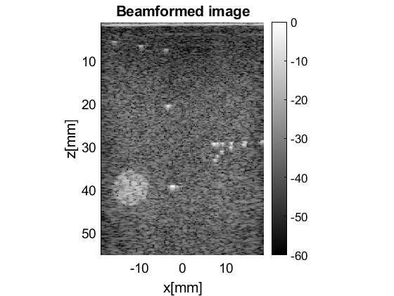
And finally display the image.

b_data.plot([],'Beamformed image');

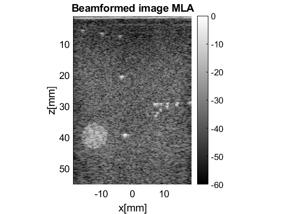
Beamforming with MLA's

MLA = 4;

scan_MLA=uff.linear_scan('x_axis',linspace(x_axis(1),x_axis(end),length(x_axis)*MLA)','z_axis',z_axis);

mid_MLA=midprocess.das();
mid_MLA.dimension = dimension.both();

mid_MLA.channel_data=channel_data;
mid_MLA.scan=scan_MLA;

mid_MLA.transmit_apodization.window=uff.window.scanline;
% We are using the hybrid transmit delay model. See the reference below:
% Rindal, O. M. H., Rodriguez-Molares, A., & Austeng, A. (2018). A simple , artifact-free , virtual source model.
% IEEE International Ultrasonics Symposium, IUS, 1–4.
mid_MLA.spherical_transmit_delay_model = spherical_transmit_delay_model.hybrid;
mid_MLA.transmit_apodization.MLA = MLA;
mid_MLA.transmit_apodization.MLA_overlap = 1;

mid_MLA.receive_apodization.window=uff.window.tukey25;
mid_MLA.receive_apodization.f_number=1.7;

b_data_MLA=mid_MLA.go();
b_data_MLA.plot([],'Beamformed image MLA');

USTB General beamformer MEX v1.1.2 .............done!