STA simulation on a phased array with the USTB built-in Fresnel simulator

In this example we show how to use the built-in fresnel simulator in USTB to generate a Synthetic Transmit Aperture (STA) dataset for a phased array and a sector scan and how it can be beamformed with USTB.

This tutorial assumes familiarity with the contents of the 'CPWC simulation with the USTB built-in Fresnel simulator' tutorial. Please feel free to refer back to that for more details.

% by Alfonso Rodriguez-Molares alfonso.r.molares@ntnu.no and Arun Asokan Nair anair8@jhu.edu 14.03.2017

Contents

Close all previously opened plots.

close all;

Phantom

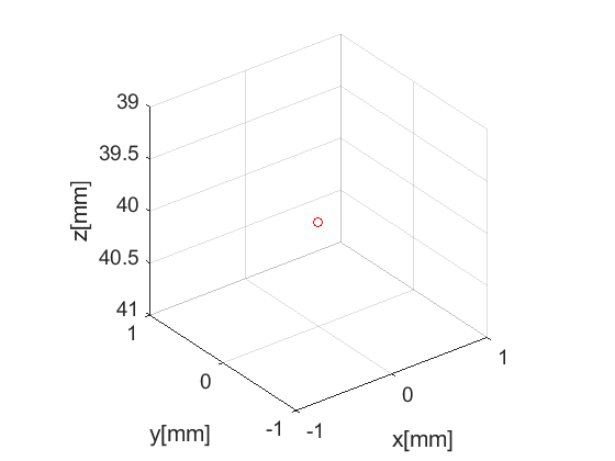
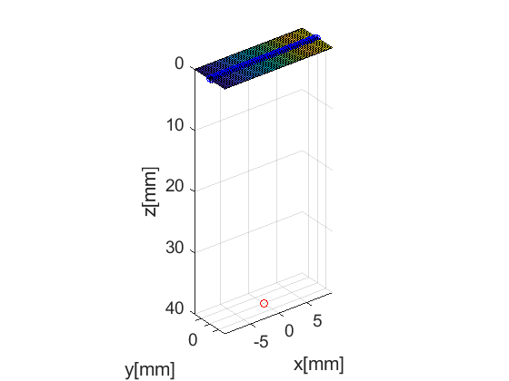
We start off defining an appropriate phantom structure to image. Our phantom here is simply a single point scatterer. USTB's implementation of phantom comes with a plot method to visualize the phantom for free!

pha=uff.phantom();
pha.sound_speed=1540;            % speed of sound [m/s]
pha.points=[0,  0, 40e-3, 1];    % point scatterer position [m]
fig_handle=pha.plot();

Probe

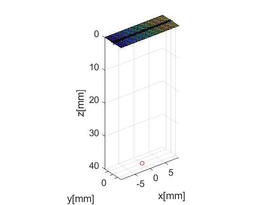
The next UFF structure we look at is probe. It contains information about the probe's geometry. USTB's implementation of probe comes with a plot method too. When combined with the previous figure we can see the position of the probe respect to the phantom.

prb=uff.linear_array();
prb.N=64;                   % number of elements
prb.pitch=300e-6;           % probe pitch in azimuth [m]
prb.element_width=270e-6;   % element width [m]
prb.element_height=7000e-6; % element height [m]
prb.plot(fig_handle);

Pulse

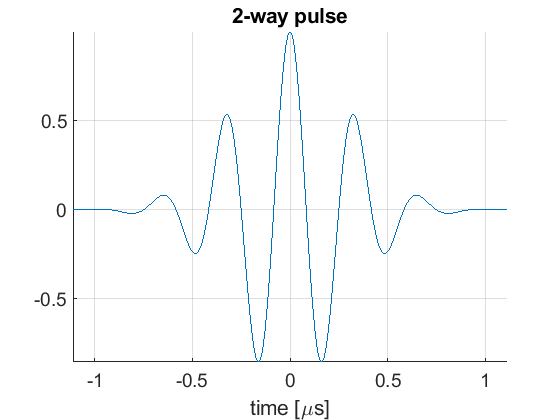
We then define the pulse-echo signal which is done here using the fresnel simulator's pulse structure. We could also use 'Field II' for a more accurate model.

pul=uff.pulse();
pul.center_frequency=3e6;       % transducer frequency [MHz]
pul.fractional_bandwidth=0.6;   % fractional bandwidth [unitless]
pul.plot([],'2-way pulse');

Sequence generation

Now, we shall generate our sequence! Keep in mind that the fresnel simulator takes the same sequence definition as the USTB beamformer. In UFF and USTB a sequence is defined as a collection of wave structures.

For our example here, we define a sequence of 64 (= number of elements) waves each emanating from a single element on the probe aperture. An appropriate apodization window is enforced through setting apodization.window = uff.window.sta. The wave structure too has a plot method.

seq=uff.wave();
for n=1:prb.N_elements
    seq(n)=uff.wave();
    seq(n).probe=prb;
    seq(n).source.xyz=[prb.x(n) prb.y(n) prb.z(n)];

    seq(n).apodization=uff.apodization();
    seq(n).apodization.window=uff.window.sta;
    seq(n).apodization.origin=seq(n).source;

    seq(n).sound_speed=pha.sound_speed;

    % show source
    fig_handle=seq(n).source.plot(fig_handle);
end

The Fresnel simulator

Finally, we launch the built-in simulator. The simulator takes in a phantom, pulse, probe and a sequence of wave structures along with the desired sampling frequency, and returns a channel_data UFF structure.

sim=fresnel();

% setting input data
sim.phantom=pha;                                % phantom
sim.pulse=pul;                                  % transmitted pulse
sim.probe=prb;                                  % probe
sim.sequence=seq;                               % beam sequence
sim.sampling_frequency=4*pul.center_frequency;  % sampling frequency [Hz]

% we launch the simulation
channel_data=sim.go();

USTB's Fresnel impulse response simulator (v1.0.7)
---------------------------------------------------------------

Scan

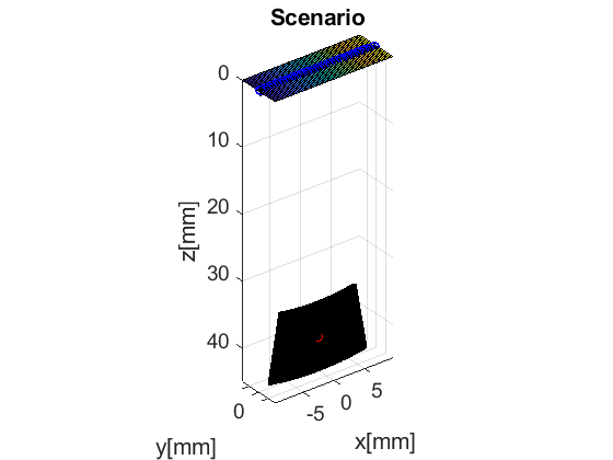
The scan area is defines as a collection of pixels spanning our region of interest. For our example here, we use the sector_scan structure, which is defined with two components: the azimuthal(angle) range and the depth(radial) range. scan too has a useful plot method it can call.

sca=uff.sector_scan('azimuth_axis',linspace(-10*pi/180,10*pi/180,200).','depth_axis', linspace(35e-3,45e-3,100).');
sca.plot(fig_handle,'Scenario');    % show mesh

Beamformer

With channel_data and a scan we have all we need to produce an ultrasound image. We now use a USTB structure beamformer, that takes an apodization structure in addition to the channel_data and scan.

pipe=pipeline();
pipe.channel_data=channel_data;
pipe.scan=sca;

pipe.receive_apodization.window=uff.window.tukey50;
pipe.receive_apodization.f_number=1.7;

pipe.transmit_apodization.window=uff.window.tukey50;
pipe.transmit_apodization.f_number=1.7;

The beamformer structure allows you to implement different beamformers by combination of multiple built-in processes. By changing the process chain other beamforming sequences can be implemented. It returns yet another UFF structure: beamformed_data.

To achieve the goal of this example, we use delay-and-sum (implemented in the das() process) as well as coherent compounding.

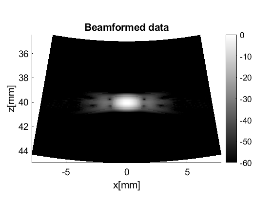
b_data=pipe.go({midprocess.das() postprocess.coherent_compounding()});

% show
b_data.plot();

USTB General beamformer MEX v1.1.2 .............done!

Published with MATLAB® R2020b