FI simulation on a phased array with the USTB built-in Fresnel simulator

In this example we show how to use the built-in fresnel simulator in USTB to generate a Conventional Focused Imaging (single focal depth) dataset for a phased array and a sector scan and show how it can be beamformed with USTB.

This tutorial assumes familiarity with the contents of the 'CPWC simulation with the USTB built-in Fresnel simulator' tutorial. Please feel free to refer back to that for more details.

by Alfonso Rodriguez-Molares alfonso.r.molares@ntnu.no and Arun Asokan Nair anair8@jhu.edu 11.03.2017

Contents

Close all previously opened plots.

close all;

Phantom

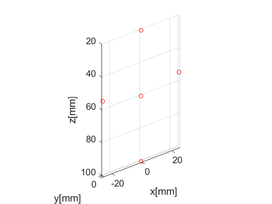
We start off defining an appropriate phantom structure to image. Our phantom here is simply a single point scatterer. USTB's implementation of phantom comes with a plot method to visualize the phantom for free!

pha=uff.phantom();
pha.sound_speed=1540;                                               % speed of sound [m/s]
[X Z] = meshgrid(0,linspace(20e-3,100e-3,3));
pha.points=[X(:),  zeros(numel(X),1), Z(:), ones(numel(X),1)];      % point scatterer position [m]
radius=60e-3;
angles=linspace(-25,25,3)*pi/180;
for n=1:length(angles)
    pha.points=[pha.points; radius*sin(angles(n)),  0, radius*cos(angles(n)), 1];    % point scatterer position [m]
end

fig_handle=pha.plot();

Probe

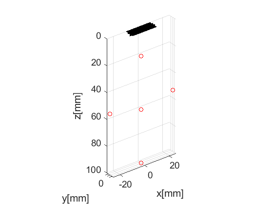
The next UFF structure we look at is probe. It contains information about the probe's geometry. USTB's implementation of probe comes with a plot method too. When combined with the previous figure we can see the position of the probe respect to the phantom.

prb=uff.linear_array();
prb.N=64;                   % number of elements
prb.pitch=300e-6;           % probe pitch in azimuth [m]
prb.element_width=270e-6;   % element width [m]
prb.element_height=7000e-6; % element height [m]
prb.plot(fig_handle);

Pulse

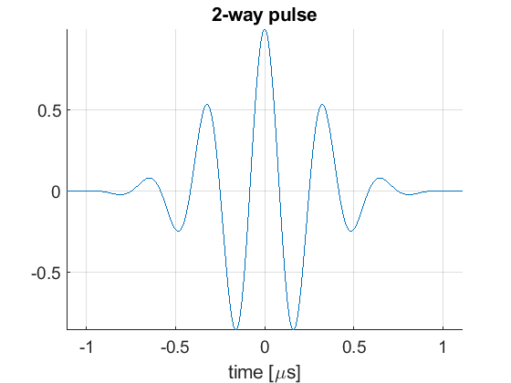
We then define the pulse-echo signal which is done here using the fresnel simulator's pulse structure. We could also use 'Field II' for a more accurate model.

pul=uff.pulse();
pul.center_frequency=3e6;       % transducer frequency [MHz]
pul.fractional_bandwidth=0.6;   % fractional bandwidth [unitless]
pul.plot([],'2-way pulse');

Sequence generation

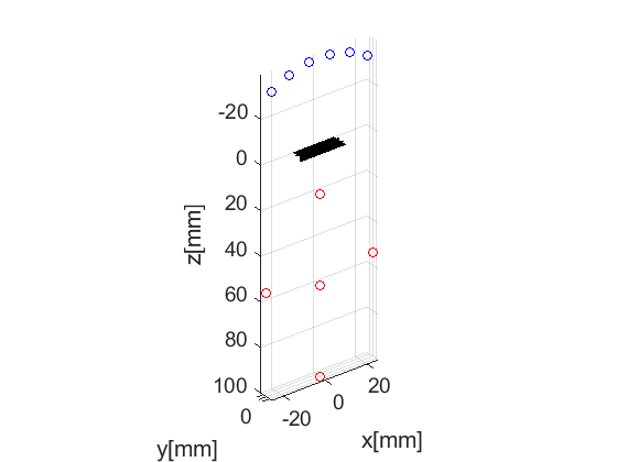
Now, we shall generate our sequence! Keep in mind that the fresnel simulator takes the same sequence definition as the USTB beamformer. In UFF and USTB a sequence is defined as a collection of wave structures.

For our example here, we define a sequence of 31 diverging waves.

N=6;                                            % number of diverging waves
azimuth_axis=linspace(-35*pi/180,35*pi/180,N).'; % beam angle vector [rad]
depth=40e-3;                                     % fixed focal depth [m]
seq=uff.wave();
for n=1:N
    seq(n)=uff.wave();
    seq(n).probe=prb;

    seq(n).source=uff.point();
    seq(n).source.azimuth=azimuth_axis(n);
    seq(n).source.distance=-depth;

    seq(n).apodization=uff.apodization();
    seq(n).apodization.window=uff.window.rectangular;
    seq(n).apodization.f_number=1.7;
    seq(n).apodization.focus=uff.sector_scan('xyz',seq(n).source.xyz);

    seq(n).sound_speed=pha.sound_speed;

    % show source
    fig_handle=seq(n).source.plot(fig_handle);
end

The Fresnel simulator

Finally, we launch the built-in simulator. The simulator takes in a phantom, pulse, probe and a sequence of wave structures along with the desired sampling frequency, and returns a channel_data UFF structure.

sim=fresnel();

% setting input data
sim.phantom=pha;                % phantom
sim.pulse=pul;                  % transmitted pulse
sim.probe=prb;                  % probe
sim.sequence=seq;               % beam sequence
sim.sampling_frequency=41.6e6;  % sampling frequency [Hz]

% we launch the simulation
channel_data=sim.go();

USTB's Fresnel impulse response simulator (v1.0.7)
---------------------------------------------------------------

Scan

The scan area is defines as a collection of pixels spanning our region of interest. For our example here, we use the sector_scan structure to generate a sector scan. scan too has a useful plot method it can call.

scan=uff.sector_scan('azimuth_axis',linspace(-35*pi/180,35*pi/180,256).','depth_axis',linspace(5e-3,110e-3,512).');

Beamformer

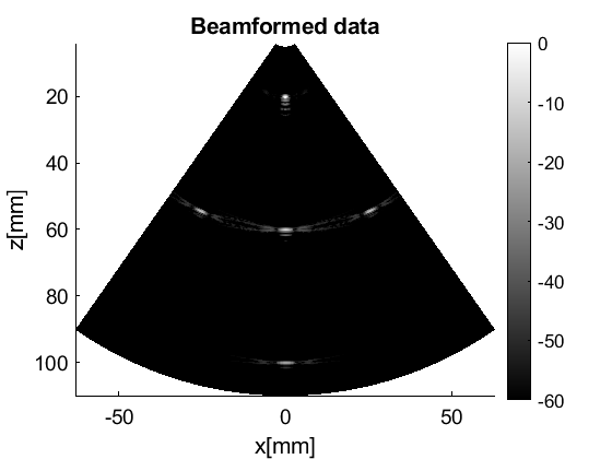
With channel_data and a scan we have all we need to produce an ultrasound image. We now use a USTB structure midprocess, that takes an apodization structure in addition to the channel_data and scan, and returns a beamformed_data.

mid=midprocess.das();
mid.dimension = dimension.both;
mid.channel_data=channel_data;
mid.scan=scan;

mid.transmit_apodization.window = uff.window.hamming;
mid.transmit_apodization.f_number=1.8;
mid.transmit_apodization.minimum_aperture = 5e-3;

mid.receive_apodization.window=uff.window.hamming;
mid.receive_apodization.f_number=1.7;

b_data=mid.go();

% show
b_data.plot();

USTB General beamformer MEX v1.1.2 .............done!

Analyse the transmit apodization used

We can plot the apodization and get a GUI to choose which pixel in the scan we want to plot the apodization across the aperture by using the transmit_apodization.plot() function. To exit press "enter".

%mid.transmit_apodization.plot([],1)

Published with MATLAB® R2020b