Computation of a CPWI dataset with Field II and beamforming with USTB
This example shows how to create a Field II simulation of Coherent Plane Wave Compounded (CPWC) imaging into a USTB channel_data object and beamform the image using the USTB routines. The Field II simulation program (field-ii.dk) should be in MATLAB's path.
date: 03.10.2017 authors: Ole Marius Hoel RIndal olemarius@olemarius.net Alfonso Rodriguez-Molares alfonso.r.molares@ntnu.no
Contents
Clear old workspace and close old plots
close all;
Basic Constants
Our first step is to define some basic constants for our imaging scenario - below, we set the speed of sound in the tissue, sampling frequency and sampling step size in time.
c0=1540;     % Speed of sound [m/s]
fs=100e6;    % Sampling frequency [Hz]
dt=1/fs;     % Sampling step [s]
field II initialisation
Next, we initialize the field II toolbox. Again, this only works if the Field II simulation program (field-ii.dk) is in MATLAB's path. We also pass our set constants to it.
field_init(0);
set_field('c',c0);              % Speed of sound [m/s]
set_field('fs',fs);             % Sampling frequency [Hz]
set_field('use_rectangles',1);  % use rectangular elements
      *------------------------------------------------------------*
      *                                                            *
      *                      F I E L D   I I                       *
      *                                                            *
      *              Simulator for ultrasound systems              *
      *                                                            *
      *             Copyright by Joergen Arendt Jensen             *
      *    Version 3.30, April 5, 2021 (Matlab 2021a version)      *
      *                  Web-site: field-ii.dk                     *
      *                                                            *
      *     This is citationware. Note the terms and conditions    *
      *     for use on the web-site at:                            *
      *               field-ii.dk/?copyright.html                  *
      *  It is illegal to use this program, if the rules in the    *
      *  copyright statement is not followed.                      *
      *------------------------------------------------------------*
Warning:  Remember to set all pulses in apertures for the new sampling frequency
Transducer definition L11-4v, 128-element linear array transducer
Our next step is to define the ultrasound transducer array we are using. For this experiment, we shall use the L11-4v 128 element Verasonics Transducer and set our parameters to match it.
probe = uff.linear_array();
f0                      = 5.1333e+06;      % Transducer center frequency [Hz]
lambda                  = c0/f0;           % Wavelength [m]
probe.element_height    = 5e-3;            % Height of element [m]
probe.pitch             = 0.300e-3;        % probe.pitch [m]
kerf                    = 0.03e-03;        % gap between elements [m]
probe.element_width     = probe.pitch-kerf;% Width of element [m]
lens_el                 = 20e-3;           % position of the elevation focus
probe.N                 = 128;             % Number of elements
pulse_duration          = 2.5;             % pulse duration [cycles]
Pulse definition
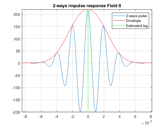
We then define the pulse-echo signal which is done here using the fresnel simulator's pulse structure. We could also use 'Field II' for a more accurate model.
pulse = uff.pulse();
pulse.fractional_bandwidth = 0.65;        % probe bandwidth [1]
pulse.center_frequency = f0;
t0 = (-1/pulse.fractional_bandwidth/f0): dt : (1/pulse.fractional_bandwidth/f0);
impulse_response = gauspuls(t0, f0, pulse.fractional_bandwidth);
impulse_response = impulse_response-mean(impulse_response); % To get rid of DC

te = (-pulse_duration/2/f0): dt : (pulse_duration/2/f0);
excitation = square(2*pi*f0*te+pi/2);
one_way_ir = conv(impulse_response,excitation);
two_way_ir = conv(one_way_ir,impulse_response);
lag = length(two_way_ir)/2+1;

% We display the pulse to check that the lag estimation is on place
% (and that the pulse is symmetric)

figure;
plot((0:(length(two_way_ir)-1))*dt -lag*dt,two_way_ir); hold on; grid on; axis tight
plot((0:(length(two_way_ir)-1))*dt -lag*dt,abs(hilbert(two_way_ir)),'r')
plot([0 0],[min(two_way_ir) max(two_way_ir)],'g');
legend('2-ways pulse','Envelope','Estimated lag');
title('2-ways impulse response Field II');

Aperture Objects
Next, we define the the mesh geometry with the help of Field II's xdc_linear_array function.
noSubAz=round(probe.element_width/(lambda/8));        % number of subelements in the azimuth direction
noSubEl=round(probe.element_height/(lambda/8));       % number of subelements in the elevation direction
Th = xdc_linear_array (probe.N, probe.element_width, probe.element_height, kerf, noSubAz, noSubEl, [0 0 Inf]);
Rh = xdc_linear_array (probe.N, probe.element_width, probe.element_height, kerf, noSubAz, noSubEl, [0 0 Inf]);

% We also set the excitation, impulse response and baffle as below:
xdc_excitation (Th, excitation);
xdc_impulse (Th, impulse_response);
xdc_baffle(Th, 0);
xdc_center_focus(Th,[0 0 0]);
xdc_impulse (Rh, impulse_response);
xdc_baffle(Rh, 0);
xdc_center_focus(Rh,[0 0 0]);
Define plane wave sequence
Define the start_angle and number of angles
F_number = 1.7;
alpha_max = atan(1/2/F_number);
Na=15;                                      % number of plane waves
F=1;                                        % number of frames
alpha=linspace(-alpha_max,alpha_max,Na);    % vector of angles [rad]
Define phantom
Define some points in a phantom for the simulation
point_position(1,:) = [0 0 10e-3];
point_position(2,:) = [-5e-3 0 10e-3];
point_position(3,:) = [5e-3 0 10e-3];
point_position(4,:) = [0 0 15e-3];

% Set point amplitudes
point_amplitudes = ones(size(point_position,1),1);
output data
cropat=round(2*50e-3/c0/dt);    % maximum time sample, samples after this will be dumped
CPW=zeros(cropat,probe.N,Na,F);  % impulse response channel data
Compute CPW signals
time_index=0;
disp('Field II: Computing CPW dataset');
wb = waitbar(0, 'Field II: Computing CPW dataset');
for f=1:F
    waitbar(0, wb, sprintf('Field II: Computing CPW dataset, frame %d',f));
    for n=1:Na
        waitbar(n/Na, wb);
        disp(['Calculating angle ',num2str(n),' of ',num2str(Na)]);

        % transmit aperture
        xdc_apodization(Th,0,ones(1,probe.N));
        xdc_times_focus(Th,0,probe.geometry(:,1)'.*sin(alpha(n))/c0);

        % receive aperture
        xdc_apodization(Rh, 0, ones(1,probe.N));
        xdc_focus_times(Rh, 0, zeros(1,probe.N));

        % do calculation
        [v,t]=calc_scat_multi(Th, Rh, point_position, point_amplitudes);

        % build the dataset
        CPW(1:size(v,1),:,n,f)=v;

        % Save transmit sequence
        seq(n)=uff.wave();
        seq(n).probe=probe;
        seq(n).source.azimuth=alpha(n);
        seq(n).source.distance=Inf;
        seq(n).sound_speed=c0;
        seq(n).delay = -lag*dt+t;
    end
end
close(wb);
Index exceeds the number of array elements (1).

Error in CPWC_L11_probe_sim (line 127)
disp('Field II: Computing CPW dataset');
Channel Data
In this part of the code, we creat a uff data structure to specifically store the captured ultrasound channel data.
channel_data = uff.channel_data();
channel_data.sampling_frequency = fs;
channel_data.sound_speed = c0;
channel_data.initial_time = 0;
channel_data.pulse = pulse;
channel_data.probe = probe;
channel_data.sequence = seq;
channel_data.data = CPW./max(CPW(:));
Scan
The scan area is defines as a collection of pixels spanning our region of interest. For our example here, we use the linear_scan structure, which is defined with two components: the lateral range and the depth range. scan too has a useful plot method it can call.
sca=uff.linear_scan('x_axis',linspace(-10e-3,10e-3,256).', 'z_axis', linspace(5e-3,20e-3,256).');
Pipeline
With channel_data and a scan we have all we need to produce an ultrasound image. We now use a USTB structure pipeline, that takes an apodization structure in addition to the channel_data and scan.
pipe=pipeline();
pipe.channel_data=channel_data;
pipe.scan=sca;

pipe.receive_apodization.window=uff.window.tukey25;
pipe.receive_apodization.f_number=F_number;
The pipeline structure allows you to implement different beamformers by combination of multiple built-in processes. By changing the process chain other beamforming sequences can be implemented. It returns yet another UFF structure: beamformed_data.
To achieve the goal of this example, we use delay-and-sum (implemented in the das_mex() process) as well as coherent compounding.
b_data=pipe.go({midprocess.das() postprocess.coherent_compounding()});

% Display images
b_data.plot();
Save UFF dataset
Finally, we can save the data into a UFF file.
channel_data.write([ustb_path(),'/data/FieldII_CPWC_simulation_v2.uff'],'channel_data');